14PhysicalDWDesign

Physical Data Warehouse Design

Outline

Techniques for Physical Data Warehouse Design
Materialized View
Indexes for Data Warehouses
Evaluation of Star Queries
Data Warehouse Partitioning

Physical data warehouse design involves implementing the logical data model and determining how data is stored, indexed, and organized for optimal query performance.

The primary goal is to make data retrieval fast and efficient for analytical purposes.

Three key techniques for achieving this are materialized views, indexing, and partitioning.

A materialized view is a database object that stores the pre-computed results of a query. Unlike a standard view, which is a virtual table defined by a query, a materialized view is a physical table that contains data. This is particularly useful in data warehousing because complex, time-consuming queries (like those involving joins and aggregations) can be executed once and their results stored, ready for rapid access.

Indexing is a data structure technique used to speed up data retrieval operations on a database table. In a data warehouse, where queries often involve complex joins and filters on large datasets, specialized indexes are crucial.

Partitioning is the process of dividing a large relational table or index into smaller, more manageable pieces called partitions. These partitions are stored separately, which can improve query performance and data maintenance.

Techniques for Physical Data Warehouse Design

Materialized Views
- A view physically stored in the DB
- Typical problems: view update, view selection
Indexing
- Used in Data Warehouse together with materialized views
- Specific for Data Warehouse: bitmap and join indexes
Partitioning
- Divides the contents of a relational table into several files
- Horizontal and vertical partitioning

Physical Data Warehouse Design

Outline

Techniques for Physical Data Warehouse Design
Materialized View
Indexes for Data Warehouses
Evaluation of Star Queries
Data Warehouse Partitioning

Materialized views improve query performance by storing the results of a query, eliminating the need to recompute data for complex queries.

The two primary methods for using them are the brute force method and transparent query rewrite.

In the brute force method, a SQL query is written to explicitly reference the materialized view by name. This means the developer or user must know the materialized view exists and must specifically include it in their query's FROM clause.

Pros: It's straightforward and gives the user full control over which view to use.

Cons: It requires a change to the application code, and the query is no longer flexible if a better view becomes available or if the materialized view is dropped.

Instead of a complex query joining sales, products, and stores tables, a user would write:

SELECT product_name, store_name, sum_sales FROM my_materialized_view;

Transparent query rewrite is a more sophisticated and powerful method. It is a feature of the database's query optimizer that automatically and intelligently redirects a user's query to a suitable materialized view, without the user's knowledge or intervention.

The query optimizer analyzes the original query (which still references the base tables) and determines if the same result can be obtained more efficiently by accessing a materialized view. If it can, the optimizer "rewrites" the execution plan to use the materialized view instead of the underlying base tables.

Pros: Application-agnostic: It doesn't require any changes to existing application code. Developers can add or remove materialized views like indexes to tune performance without impacting the application.

Efficiency: The optimizer can choose the best materialized view among several options to satisfy the query, based on what it determines to be the most efficient path.

Cons: Not always guaranteed: The optimizer may not always be able to perform a rewrite, especially if the query is very complex or if the materialized view's data is not fresh enough to satisfy the query's requirements.

Requires configuration: The feature must be enabled in the database, and the materialized views must be configured to be eligible for query rewrite.

Example:

A user submits the original, complex query:

SELECT P.product_name, S.store_name, SUM(T.total_sales) FROM sales T JOIN products P ON T.prod_id = P.id JOIN stores S ON T.store_id = S.id GROUP BY P.product_name, S.store_name;

The query optimizer sees that the my_materialized_view contains the exact pre-computed result of this join and aggregation. It transparently re-routes the query to use the view, and the user receives the results quickly, unaware that the underlying query plan was changed.

Materialized Views

Materialized view is a relational table that contains the rows that would be returned by the view definition - usually SELECT statement of SQL
If we consider relational views as stored queries then materialized views can be considered as stored results
Materialized views are created and used to reduce an amount of time needed to compute SELECT statements, for example join materialized views eliminate the needs to join the relational table
There are two ways how materialized view can be used:
- brute force method
- transparent query rewrite
In brute force method SQL is written to explicitly access the view
Transparent query rewrite method is applied when a query optimizer detects that a query can be computed against a materialized view instead of the source relational tables

View maintenance is the process of keeping a materialized view synchronized with its base tables.

Since a materialized view stores pre-computed results, any changes to the original data (insertions, deletions, or updates) require the view to be refreshed to remain accurate.

Incremental view maintenance is a highly efficient technique for this process. Instead of re-computing the entire view from scratch (a costly operation known as a complete refresh), incremental maintenance applies only the changes made to the base tables. For example, if a new row is added to a base table, the system calculates the impact of that single addition and updates the materialized view accordingly. This is much faster and less resource-intensive than re-running the full query on the entire dataset.

The provided SQL code demonstrates how to create a materialized view in Oracle Database.

CREATE MATERIALIZED VIEW MV_ORDERS

REFRESH ON COMMIT

ENABLE QUERY REWRITE

( SELECT O_ORDERKEY, O_CUSTKEY, O_TOTALPRICE, O_ORDERDATE

FROM ORDERS

TO_DATE('31-DEC-1986','DD-MON-YYYY') );>

CREATE MATERIALIZED VIEW MV_ORDERS: This statement initiates the creation of a materialized view named MV_ORDERS.

REFRESH ON COMMIT: This clause specifies that the view should be updated incrementally whenever a transaction that modifies the base table (ORDERS) is committed. This ensures the view is always up-to-date.

ENABLE QUERY REWRITE: This is a crucial setting that allows the database's query optimizer to use transparent query rewrite. When a user runs a query against the original ORDERS table, the optimizer can transparently redirect the query to the materialized view if it determines the view can provide the results more efficiently.

AS (SELECT ...): This defines the query whose results will be stored in the materialized view. In this case, it's a subset of the ORDERS table containing orders placed after December 31, 1986.

The following SQL query shows how a user can directly access the materialized view:

SQL

SELECT * FROM MV_ORDERS WHERE O_ORDERDATE = TO_DATE('01-JAN-1992','DD-MON-YYYY')

This is the brute force method. The user explicitly queries the materialized view MV_ORDERS to retrieve the desired data. This is typically done when the user knows the view exists and wants to ensure they are getting the pre-computed results, bypassing the original base table entirely.

Materialized Views

View maintenance means that when the base relational tables are updated then a materialized view must be updated too
Incremental view maintenance means that updated view is computed from the individual modifications to the relational tables and not from the entire relational tables

Creating materialized view

	      
CREATE MATERIALIZED VIEW MV_ORDERS
REFRESH ON COMMIT
ENABLE QUERY REWRITE
AS( SELECT O_ORDERKEY, O_CUSTKEY, O_TOTALPRICE, O_ORDERDATE 
    FROM ORDERS
    WHERE O_ORDERDATE > TO_DATE('31-DEC-1986','DD-MON-YYYY') );

Direct access to materialized view

	      
SELECT * 
FROM MV_ORDERS 
WHERE O_ORDERDATE = TO_DATE('01-JAN-1992','DD-MON-YYYY')

Access to a materialized view through query rewriting is a powerful database feature where the system's query optimizer automatically and transparently uses a materialized view to satisfy a query that was originally written against the base tables.

The provided SQL query SELECT O_ORDERKEY, O_CUSTKEY, O_TOTALPRICE, O_ORDERDATE FROM ORDERS WHERE O_ORDERDATE > TO_DATE('31-DEC-1986','DD-MON-YYYY'); is written to retrieve data directly from the ORDERS table.

However, the EXPLAIN PLAN output shows that the database did not access the ORDERS table. Instead, it performed a full table scan (ACCESS FULL) on the MV_ORDERS materialized view. This is a perfect example of transparent query rewriting.

The query optimizer, being intelligent, recognized that:

A materialized view named MV_ORDERS exists.

This materialized view contains the exact data needed to satisfy the query.

Accessing the MV_ORDERS materialized view is more efficient than scanning the large ORDERS table and filtering the rows.

As a result, it transparently rewrote the execution plan to use the materialized view. The user wrote a query on the base table, but the database executed it against the materialized view, resulting in much faster performance without any changes to the user's code.

The Predicate Information section of the EXPLAIN PLAN confirms this by showing that the filter condition O_ORDERDATE > TO_DATE('1986-12-31 ...') was applied directly to the MV_ORDERS materialized view, proving that the query was indeed executed against the view.

Materialized Views

Access to materialized view through query rewriting

	      
SELECT O_ORDERKEY, O_CUSTKEY, O_TOTALPRICE, O_ORDERDATE 
FROM ORDERS
WHERE O_ORDERDATE > TO_DATE('31-DEC-1986','DD-MON-YYYY');

The results from EXPLAIN PLAN statement


PLAN_TABLE_OUTPUT 
----------------------------------------------------------------------------------
| 0  | SELECT STATEMENT            |           | 108K| 2539K| 507 (1)| 00:00:01 | 
|* 1 | MAT_VIEW REWRITE ACCESS FULL| MV_ORDERS | 108K| 2539K| 507 (1)| 00:00:01 | 
---------------------------------------------------------------------------------- 
Predicate Information (identified by operation id):
1 - filter("MV_ORDERS"."O_ORDERDATE">TO_DATE(' 1986-12-31 00:00:00', 
           'syyyy-mm-dd hh24:mi:ss'))

Physical Data Warehouse Design

Outline

Techniques for Physical Data Warehouse Design
Materialized View
Indexes for Data Warehouses
Evaluation of Star Queries
Data Warehouse Partitioning

An index is a data structure that improves the speed of data retrieval operations on a database table.

It works like the index of a book, allowing the database to quickly find specific data without having to scan every single row in the table.

When you execute a query like SELECT * FROM EMPLOYEE WHERE EmployeeKey = 007;, without an index on the EmployeeKey column, the database would have to perform a full table scan. This means it would sequentially read every row in the EMPLOYEE table, checking if the EmployeeKey matches '007'. For a large table, this is a slow and resource-intensive process.

However, if there's an index on EmployeeKey, the database can use it to pinpoint the exact location of the record. This typically involves just a few disk block accesses, which is significantly faster than a full scan.

Drawbacks of Indexes

While indexes are great for speeding up data retrieval, they aren't without their downsides:

Update overhead: Every time you INSERT, UPDATE, or DELETE a row in a table with an index, the index itself must be updated to reflect the change. This adds overhead and can slow down write operations.

Storage cost: Indexes are separate data structures that consume disk space.

Performance degradation: Too many indexes on a single table can lead to degraded performance, especially for write-heavy workloads, due to the cumulative maintenance overhead.

Popular Indexing Techniques

The two most common indexing techniques in relational databases are B*-trees and bitmap indexes.

B*-trees: These are the default and most widely used index type. They are well-suited for high-cardinality columns, such as a unique primary key like EmployeeKey. B*-trees are a balanced, tree-like data structure that provides fast access for both exact matches and range queries.

Bitmap indexes: Unlike B*-trees, bitmap indexes are best for low-cardinality columns, meaning columns with a small number of distinct values (e.g., gender, marital status, or country code). They use a bit array for each distinct value, which makes it very efficient to combine multiple conditions using logical operations (AND, OR) directly on the bitmaps. They are particularly popular in data warehouses where read-heavy, analytical queries are common.

Indexes for Data Warehouses

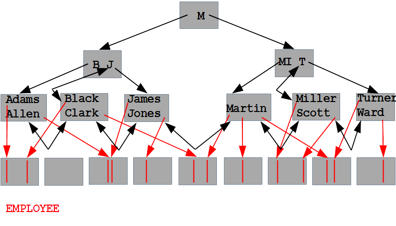
An index provides a quick way to locate data of interest

Sample query

	      
SELECT *
FROM EMPLOYEE
WHERE EmployeeKey = 007;

With the help of an index over a column EmployeeKey (primary key in EMPLOYEE table), a single disk block access will suffice to answer the query
Without this index, we should perform a complete scan of table EMPLOYEE
Drawback: Almost every update on an indexed attribute also requires an index update
Too many indexes may degrade performance
Most popular indexing techniques in relational databases include B*-trees and bitmap indexes

A B*-tree is a type of search tree specifically designed for disk-based storage systems, where disk I/O operations are very expensive. Its structure minimizes the number of disk reads required to find, insert, or delete data. Unlike a simple binary tree, B*-tree nodes can hold many keys and have a high fanout (many children).

The traversal of a B*-tree is a combination of two methods to get data in sorted order:

Vertical Traversal (from root to leaf): This is the primary traversal method for searching. To find a specific key, the search starts at the root node and moves down through the tree. At each internal node, the algorithm efficiently determines which child subtree to follow by comparing the search key to the keys stored in the current node. This process continues until the search reaches a leaf node. Since all leaf nodes in a B*-tree are at the same level, this ensures a consistent search time.

Horizontal Traversal (at the leaf level): Once the search has found a particular key, it can then traverse the data horizontally. The leaf nodes of a B*-tree are linked together in a sequential, sorted order. This "horizontal" link allows for efficient sequential access to data, such as retrieving all records in a certain range, without having to go back up the tree. You can traverse from the left-most leaf to the right-most, or vice versa, to get the data in sorted order.

Therefore, the combined method is vertically from the root to the leaf level to find the starting point, and then horizontally at the leaf level to retrieve the data of interest. This makes B*-trees incredibly efficient for both single-record lookups and large-scale data scans.

B*-tree index implementation

ORM

B*-tree can be traversed either:
- vertically from root to leaf level of a tree
- horizontally either from left corner of leaf level to right corner of leaf level or the opposite
- vertically and later on horizontally either towards left lower corner or right lower corner of leaf level

A bitmap index is a special type of database index that is highly effective for columns with low cardinality, which means the column has a small number of distinct values. Examples include columns like gender (Male/Female) or status (Active/Inactive).

Instead of storing pointers to individual rows for each value, a bitmap index creates a separate bitmap (a bit array) for each distinct value in the indexed column.

Each bit in the bitmap corresponds to a single row in the table.

A 1 indicates that the row contains the value associated with the bitmap.

A 0 indicates that it doesn't.

For a gender column with Male and Female as distinct values, a bitmap index would create two bitmaps: one for "Male" and one for "Female."

The "Male" bitmap would have a 1 for every row where gender is "Male."

The "Female" bitmap would have a 1 for every row where gender is "Female."

The real power of bitmap indexes comes from how they handle complex queries. When a query includes multiple conditions, such as WHERE gender = 'Male' AND status = 'Active', the database can perform bitwise logical operations (like AND or OR) directly on the bitmaps. This is extremely fast because these operations are handled at a very low level by the CPU. The result is a new bitmap that points to the exact rows that satisfy all the conditions, avoiding a full table scan and dramatically speeding up the query.

Benefits:

High Performance: Very fast for read-heavy analytical queries, especially those with multiple WHERE conditions.

Space Efficient: For low-cardinality columns, bitmaps are very compact.

Efficient for Ad-Hoc Queries: Great for data warehouses and business intelligence where queries are often complex and unpredictable.

Drawbacks:

Updatawbacks:

Update Overhead: They are not suitable for transactional systems with frequent updates, inserts, or deletions, as modifying a single row requires updating the entire bitmap, which can be slow.

High Cardinality Issues: For columns with many distinct values, such as a primary key, a bitmap index would be inefficient and large, as it would need to create a bitmap for every unique value.

Bitmap Indexes

To process a query for products with a specific range of pieces per unit and unit price using a bitmap index, the database performs bitwise operations on the bitmaps. This is far more efficient than scanning the entire table.

The query is: SELECT * FROM Products WHERE PiecesPerUnit BETWEEN 45 AND 55 AND UnitPrice BETWEEN 100 AND 200.

The database will follow these steps:

Retrieve Relevant Bitmaps: The database fetches the bitmaps for each condition in the WHERE clause.

For PiecesPerUnit BETWEEN 45 AND 55: It retrieves the bitmaps for pieces per unit 45, 46, 47, ..., up to 55.

For UnitPrice BETWEEN 100 AND 200: It retrieves the bitmaps for unit prices 100, 101, 102, ..., up to 200.

Perform Bitwise OR Operations: The database combines the bitmaps for each range using a bitwise OR operation.

PiecesPerUnit_range_bitmap = (bitmap_45 OR bitmap_46 OR ... OR bitmap_55)

UnitPrice_range_bitmap = (bitmap_100 OR bitmap_101 OR ... OR bitmap_200)

Perform Bitwise AND Operation: Because the query uses an AND operator, the database performs a bitwise AND on the two resulting range bitmaps.

Final_result_bitmap = PiecesPerUnit_range_bitmap AND UnitPrice_range_bitmap

A bit in the Final_result_bitmap will be 1 only if the corresponding row satisfies both conditions.

Fetch the Data: Finally, the database uses the Final_result_bitmap to identify and retrieve the rows that have a 1 in the bitmap. This allows it to directly access the relevant data without scanning the entire Products table.

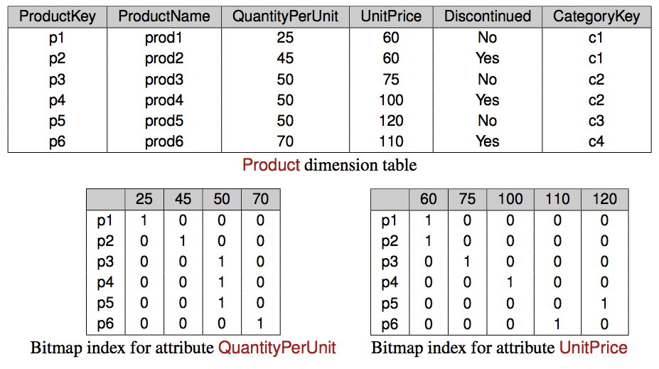
Bitmap Indexes: Example

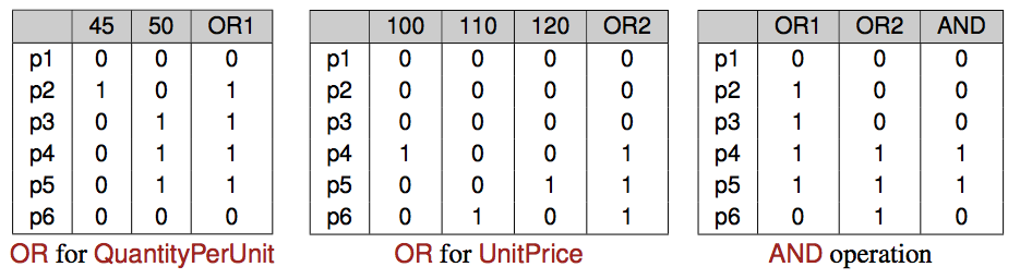
Products having between 45 and 55 pieces per unit, and with a unit price between 100 and 200

Bitmap Indexes

Symmetric Partial Match Queries

Symmetric partial match queries are a type of database query where the goal is to search across multiple dimensions of a data cube simultaneously. The term "symmetric" means that all dimensions are treated equally; any combination of dimensions can be used in a search. To handle this efficiently, all dimensions of the cube should be symmetrically indexed. This allows the database to quickly find data regardless of which dimensions are used in the search criteria. A good example of an indexing technique that supports this is a join index, which can pre-compute joins on multiple dimensions.

Indexing at Multiple Levels of Aggregation

In data warehousing, data is often aggregated into summary tables to speed up queries. Indexing at multiple levels of aggregation means that these summary tables must be indexed in the same way as the base, unaggregated tables. This ensures that queries against the summary tables, which are common for high-level analysis, are as fast as possible. For example, if you have a base Sales table and a Monthly_Sales_Summary table, both should have similar indexing on their key dimensions (e.g., product, store, and time) to enable quick lookups at different levels of detail.

Efficient Batch Update

Efficient batch update refers to the process of refreshing a data warehouse with new data, which is typically done in large batches (e.g., nightly). The indexing schema must be designed with this in mind. The refreshing time of a data warehouse must be considered when designing the indexing schema. Too many indexes, or complex indexes like bitmap indexes, can significantly slow down the loading process. Therefore, a balance must be struck between optimizing for fast queries and minimizing the time required to refresh the data. The chosen indexing strategy should allow for quick updates, or it should be possible to disable and re-enable indexes during the update process.

Sparse Data

Sparse data is a common issue in data cubes, where a large number of possible combinations of dimension values do not have any corresponding data. For instance, a cell representing the sale of a specific product in a specific store on a specific day may be empty if no such transaction occurred. Typically, only 20% of the cells in a data cube are nonempty. The indexing schema must be able to deal with both sparse (empty) and nonsparse (nonempty) data efficiently. Indexes like bitmap indexes, while excellent for low-cardinality data, can be inefficient for sparse data if not handled correctly. Techniques like bitmap join indexes are often used to combine the benefits of bitmap indexes with the ability to handle sparse data by indexing only the non-null values.

Indexes for Data Warehouses: Requirements

Symmetric partial match queries
- All dimensions of the cube should be symmetrically indexed, to be searched simultaneously
Indexing at multiple levels of aggregation
- Summary tables must be indexed in the same way as base nonaggregated tables
Efficient batch update
- The refreshing time of a data warehouse must be considered when designing the indexing schema
Sparse data
- Typically, only 20% of the cells in a data cube are nonempty
- The indexing schema must deal efficiently with sparse and nonsparse data

Physical Data Warehouse Design

Outline

Techniques for Physical Data Warehouse Design
Materialized View
Indexes for Data Warehouses
Evaluation of Star Queries
Data Warehouse Partitioning

Star queries are a type of database query that operates on a star schema, a common data warehousing model. In a star schema, a central fact table connects to multiple dimension tables. Star queries are named for the star-like shape of this schema. They involve joining the central fact table with one or more of its dimension tables to retrieve and analyze data.

A typical star query, like the one you provided, aims to answer a business question by combining information from different tables. Let's break down the query:

SELECT ProductName, CustomerName, SUM(SalesAmount) FROM Sales S, Customer C, Product P WHERE S.CustomerKey = C.CustomerKey AND S.ProductKey = P.ProductKey AND P.Discontinued = 'Yes' GROUP BY C.CustomerName, P.ProductName;

This query retrieves the total sales of discontinued products, broken down by customer and product.

Sales S is the fact table, containing a row for each sale and linking to the other tables.

Customer C and Product P are dimension tables, providing descriptive information about customers and products, respectively.

S.CustomerKey = C.CustomerKey and S.ProductKey = P.ProductKey are the join conditions, linking the fact table to its dimension tables.

P.Discontinued = 'Yes' is a selection condition, filtering the data to only include sales of discontinued products.

SUM(SalesAmount) and GROUP BY are the aggregation, calculating the total sales for each unique combination of customer and product that meets the criteria.

Three Steps to Evaluate a Star Query

The three steps you listed are a common way to evaluate a star query efficiently:

Evaluation of the Join Conditions: The query processor first establishes the connections between the fact table and the dimension tables. It matches the foreign keys in the fact table (e.g., S.CustomerKey) with the primary keys in the dimension tables (e.g., C.CustomerKey). This step logically links the sales data to the corresponding customer and product details.

Evaluation of the Selection Conditions: After joining the tables, the query applies the filters specified in the WHERE clause. In the example, it would filter for all rows where the product's Discontinued status is 'Yes'. This significantly reduces the number of rows that need to be processed further, making the query more efficient.

Aggregation of the Tuples: Finally, the query aggregates the filtered data. The GROUP BY clause sorts the data by CustomerName and ProductName, and then the SUM(SalesAmount) function calculates the total sales for each group. This produces the final, summarized result that answers the business question.

Star Queries

Queries over star schemas are called star queries
Join the fact table with the dimension tables

A typical star query: total sales of discontinued products, by customer name and product name

	      
SELECT ProductName, CustomerName, SUM(SalesAmount)
FROM Sales S, Customer C, Product P
WHERE S.CustomerKey = C.CustomerKey AND S.ProductKey = P.ProductKey AND
      P.Discontinued = 'Yes'
GROUP BY C.CustomerName, P.ProductName;

Three basic steps to evaluate the query:
- (1) Evaluation of the join conditions
- (2) Evaluation of the selection conditions over the dimensions
- (3) Aggregation of the tuples that passed the filter

Evaluation of Star Queries with Bitmap Indexes: Example

Bitmap Indexes

Evaluating a star query efficiently requires specific data structures. The two key structures mentioned are B+ trees and bitmap indexes, which optimize different parts of the query.

Data Structures for Star Query Evaluation

B+ tree over CustomerKey and ProductKey: A B+ tree is a tree data structure that keeps data sorted and allows for efficient searches, insertions, and deletions. In this context, B+ trees are used on the CustomerKey and ProductKey to quickly locate dimension table records (e.g., to find the customer name for a given CustomerKey). They are particularly useful for finding individual records based on a key value.

Bitmap indexes on Sales and Product tables: A bitmap index is a specialized index that uses bit arrays (vectors of 0s and 1s) to efficiently answer queries.

Bitmap indexes on foreign key columns in Sales: A bitmap is created for each distinct foreign key value (e.g., for each ProductKey like p1, p2, p3, etc.). The bit vector has a 1 at the position corresponding to a row in the fact table that contains that specific foreign key value, and a 0 otherwise. This allows for rapid identification of fact table rows that link to a specific dimension record.

Bitmap index on Discontinued in Product: This is a simple bitmap index with two bit vectors, one for 'Yes' and one for 'No', to quickly identify all products that are discontinued.

Step-by-Step Query Evaluation Using Indexes

Let's trace the query's evaluation using these indexes:

Obtain Record Numbers for Discontinued = 'Yes': The query first uses the bitmap index on Discontinued in the Product table. This immediately returns a bit vector indicating which Product records have Discontinued = 'Yes'. The corresponding ProductKey values are then identified (e.g., p2, p4, p6). This is a highly efficient way to filter a dimension table.

Perform Join Using Bitmap Vectors: Instead of a traditional join, the database uses the bitmap indexes on the foreign key columns of the Sales table. It retrieves the bitmap vectors for the ProductKey values identified in the previous step (p2, p4, p6). The database then performs a logical OR operation on these vectors to get a final bitmap that represents all fact table rows that correspond to a discontinued product.

Find Corresponding Fact Records: The combined bitmap from step 2 is then used to directly access the relevant rows in the Sales fact table. The example shows that the vectors for p2 and p4 match (i.e., there are sales records for these products), while p6 has no corresponding sales records, so it's excluded from further processing.

Obtain Customer Keys: From the sales records that match the bitmap, the CustomerKey values are extracted. In the example, these are c2 and c3.

Use B+ Tree to Get Names: The B+ tree indexes on CustomerKey and ProductKey are then used to look up the corresponding CustomerName and ProductName from the Customer and Product tables respectively. This is a fast way to get the descriptive information for the final output.

Final Result: The final results are assembled by joining the aggregated sales data with the names found in the previous step, resulting in the final output: (cust2, prod2, 200) and (cust3, prod4, 100). This demonstrates how B+ trees and bitmap indexes work together to evaluate a star query efficiently.

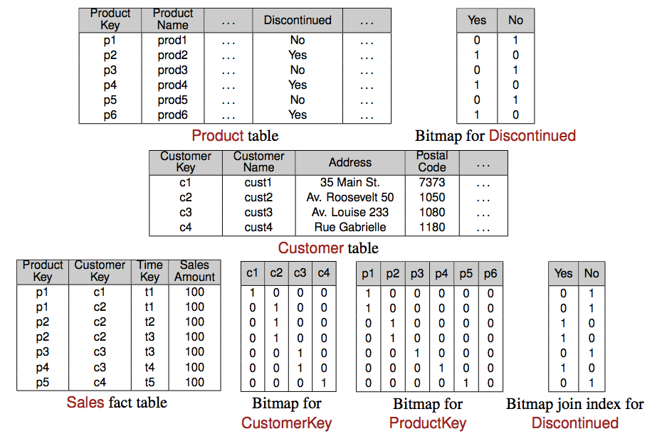
Evaluation of Star Queries using Bitmap Indexes

Evaluation of star query requires
- a B+ tree over CustomerKey and ProductKey
- Bitmap indexes on the foreign key columns in Sales and on Discontinued in Product
Example of query evaluation
- (1) Obtain the record numbers of the records that satisfy the condition Discontinued = 'Yes'
- Answer: Records with ProductKey values p2 , p4 , and p6
- (2) To access the bitmap vectors in Sales with these labels perform a join between Product and Sales
- (3) Vectors labeled p2 and p4 match, no fact record for p6
- (4) Obtain the values for the CustomerKey in these records (c2 andc3 )
- (5) Use B+-tree index on ProductKey and CustomerKey to find the names of products and customers
- (6) Answer: (cust2,prod2,200) and (cust3,prod4,100)

Physical Data Warehouse Design

Outline

Techniques for Physical Data Warehouse Design
Materialized View
Indexes for Data Warehouses
Evaluation of Star Queries
Data Warehouse Partitioning

Partitioning, or fragmentation, is a database technique used to divide a large table or index into smaller, more manageable pieces called partitions. This improves performance, manageability, and availability by breaking up a single large dataset. There are two main types: vertical and horizontal partitioning.

Vertical partitioning splits a table by its columns. Instead of having one wide table with many attributes, you create two or more narrower tables, with each containing a subset of the original columns. A key column (like a primary key) is included in each new table to link them back to the original logical record.

How it works: You group columns based on how they're used. For example, frequently accessed columns are placed in one partition, while less frequently accessed or very large columns (like text blobs) are stored in another.

Benefits: By reducing the number of columns in a single table, you can fit more records into memory. This reduces the amount of I/O needed to retrieve data, making queries that only access a subset of columns much faster.

Horizontal partitioning splits a table by its rows. The original table's rows are divided into several smaller tables, each with the same schema (columns) as the original but containing different subsets of the data.

How it works: You divide the data based on a specific criterion, such as a date range, geographical location, or customer ID. For example, a sales table might be partitioned horizontally so that all sales from the last quarter are in one partition, and older data is in another.

Benefits: Queries that target only a specific partition (e.g., "show me all sales from October") don't have to scan the entire table, drastically improving performance. This is especially useful for managing historical data, where old data can be moved to a separate partition and even archived on cheaper storage.

Data Warehouse Partitioning

Partitioning (or fragmentation) divides a table into smaller data sets (each one called a partition)
Applied to tables and indexes
Vendors provide several dfferent partitioning methods
Vertical partitioning splits the attributes of a table into groups that can be independently stored
- E.g., most often used attributes are stored in one partition, less often used attributes in another one
- More records fit into main memory, reducing their processing time
Horizontal partitioning divides a table into smaller tables with same structure than the full table
- For example, if some queries require the most recent data, partition horizontally according to time

Partitioning improves query performance primarily through two techniques: partition pruning and partition-wise joins. These methods allow the database to process only the relevant subsets of data, significantly reducing the amount of I/O and computation required.

Partition pruning is a query optimization technique where the database automatically skips over partitions that are not relevant to a query. This is the most common way partitioning improves performance.

How it works: When a query's WHERE clause includes a condition on the column used for partitioning, the query optimizer can determine which partitions contain the data needed and which do not. It then "prunes" (or eliminates) the irrelevant partitions from the execution plan.

Example: Imagine a Sales table partitioned by month. A query asking for sales data for "January 2026" will immediately be directed to the January2026 partition. The database avoids scanning the other 11 monthly partitions, dramatically speeding up the query. This is far more efficient than scanning a single, massive table containing all sales data.

Partitioning can also enhance join performance, particularly in data warehousing where large fact tables are joined with dimension tables.

How it works: This technique is most effective when both tables being joined are partitioned on the same join key. The database can then break down a single, large join operation into multiple, smaller joins, one for each partition. This is a form of parallel processing.

Example: If a Sales fact table is partitioned by ProductKey and a Product dimension table is also partitioned by ProductKey, the database can join the Sales_partition_1 with Product_partition_1, Sales_partition_2 with Product_partition_2, and so on. This "divide and conquer" approach is much faster than joining two huge tables in their entirety. It essentially transforms one big join into many smaller, more efficient ones that can be executed in parallel.

Queries over Partitioned Databases

Partition pruning is the typical way of improving query performance using partitioning
Example: A Sales fact table in a warehouse can be partitioned by month
A query requesting orders for a single month only needs to access the partition of such a month
Joins also enhanced by using partitioning:
- When the two tables are partitioned on the join attributes
- When the reference table is partitioned on its primary key
- Large join is broken down into smaller joins

Range, hash, and list partitioning are three common strategies for dividing a large database table into smaller, more manageable partitions. Each method uses a different logic to decide which partition a record should belong to.

Range partitioning is a strategy that maps records to partitions based on a specified range of values for a partitioning key. This is the most intuitive method and is particularly useful when the data has a natural sequential or chronological order.

How it works: You define a set of ranges for the partitioning key, and each range corresponds to a specific partition. For example, a Sales table might be partitioned by date into monthly partitions.

Best for: Time-series data is a natural candidate for range partitioning. This allows for quick queries on a specific time period by targeting only the relevant partition, a process known as partition pruning. It's also easy to manage data by adding new partitions for new time periods or dropping old ones to archive historical data.

Example: In a Sales table with a Date column, you could define a January-2012 partition to hold all records with a Date value between January 1, 2012 and January 31, 2012.

Hash partitioning uses a hashing algorithm to distribute records across a fixed number of partitions. Unlike range partitioning, which groups similar data, hash partitioning aims to spread the data out evenly.

How it works: The database applies a hashing algorithm to the partitioning key (e.g., CustomerKey or a unique ID), which generates a hash value. This value is then used to determine which partition the record belongs to, typically by using a simple modulus operation.

Best for: This method is ideal when you need to distribute data uniformly to prevent any single partition from becoming a "hotspot" with a disproportionately large amount of data or query traffic. This is a common requirement for parallel processing and load balancing across multiple storage devices. It's especially useful when there is no clear business logic for partitioning the data, or when data distribution is not based on time or a specific business attribute.

Benefits: It ensures that partitions are ideally of the same size, which helps in balancing the workload across multiple disks or servers.

List partitioning is a strategy that maps records to partitions based on a predefined list of discrete values for the partitioning key.

How it works: Each partition is explicitly assigned a set of unique values. The database places a record into a partition only if its partitioning key value matches one of the values in that partition's list.

Best for: This is used when data can be grouped by specific, known categories. Common examples include partitioning by Country, Region, or ProductType.

Example: A Customer table could be list-partitioned by the Region column, with one partition for 'Europe', another for 'Asia', and a third for 'North America'. This allows for highly efficient queries that target a specific region, such as "show me all customers from Europe.

Partitioning Strategies

Three partitioning strategies: Range partitioning, hash partitioning, and list partitioning
Range partitioning maps records to partitions based on ranges of values of the partitioning key
Time dimension is a natural candidate for range partitioning
Example: A table with a date column defined as the partitioning key
- January-2012 partition will contain rows with key values from January 1 to January 31, 2012
Hash partitioning uses a hashing algorithm over the partitioning key to map records to partitions
- Hashing algorithm distributes rows among partitions in a uniform fashion, yielding, ideally, partitions of the same size
- Typically used when partitions are distributed in several devices, and when data are not partitioned based on time

Partitioning is a powerful database technique that can be combined in different ways to create highly efficient data storage and retrieval systems. List partitioning is a fundamental method that groups data based on a predefined set of discrete values. Vendors like Oracle extend this concept with composite partitioning, which allows for a multi-level partitioning scheme, combining two different methods to achieve a more granular and flexible data distribution.

List partitioning divides a table by assigning each partition a specific list of values from the partitioning key. Unlike range partitioning, which uses continuous ranges, list partitioning is based on categorical or discrete data.

How it works: For example, you can partition a Customers table by a Region column, creating a separate partition for each continent or country. A record with a Region value of 'Europe' will be stored in the 'Europe' partition, while a record with 'Asia' goes into the 'Asia' partition.

Best for: This is ideal for scenarios where data can be grouped by a finite set of known values, like product types, geographical regions, or departments. This approach simplifies data management and allows for very fast queries that only target specific list values.

Composite partitioning combines two partitioning methods: a primary method (like range or list) and a secondary method (subpartitioning) applied to each of the primary partitions. This creates a two-level hierarchy of data organization.

How it works: A common example is range-hash partitioning.

First, the table is range-partitioned by a date column (e.g., into monthly partitions). This handles the time-series aspect of the data, a common need in data warehouses.

Second, each monthly partition is then subpartitioned using a hash algorithm on a different column, like CustomerKey.

This approach combines the strengths of both methods:

Range partitioning allows for efficient queries on specific time periods by using partition pruning.

Hash subpartitioning evenly distributes the data within each monthly partition, preventing "hot spots" (partitions with a disproportionately large amount of data or queries) and enabling parallel processing.

Composite partitioning gives database administrators more granular control over data placement and can lead to significant performance improvements for complex queries by allowing the database to prune partitions and then perform parallel operations on the subpartitions.

Partitioning Strategies

List partitioning specifies a list of values for the partitioning key
Some vendors (e.g. Oracle) support the notion of composite partitioning, combining the basic data distribution methods
Thus, a table can be range partitioned, and each partition can be subdivided using hash partitioning

References

A. VAISMAN, E. ZIMANYI, Data Warehouse Systems: Design and Implementation, Chapter 7 Physical Data Warehouse Design, Springer Verlag, 2014